LGCM Tutorial

This tutorial walks through a complete LGCM analysis. By the end, you will have:

Simulated longitudinal data with known parameters
Visualized individual trajectories
Fit and compared growth models
Interpreted the results

Workflow Overview

┌─────────────────────────────────┐
│ 1. Setup                        │
│    Load packages, set seed      │
└────────────────┬────────────────┘
                 ▼
┌─────────────────────────────────┐
│ 2. Simulate/Load Data           │
│    Wide format, check structure │
└────────────────┬────────────────┘
                 ▼
┌─────────────────────────────────┐
│ 3. Visualize                    │
│    Spaghetti plot, look first   │
└────────────────┬────────────────┘
                 ▼
┌─────────────────────────────────┐
│ 4. Fit Models                   │
│    Baseline + growth models     │
└────────────────┬────────────────┘
                 ▼
┌─────────────────────────────────┐
│ 5. Compare Models               │
│    LRT, AIC/BIC                 │
└────────────────┬────────────────┘
                 ▼
┌─────────────────────────────────┐
│ 6. Check Diagnostics            │
│    Fit indices, residuals       │
└────────────────┬────────────────┘
                 ▼
┌─────────────────────────────────┐
│ 7. Interpret Results            │
│    Parameters, effect sizes     │
└─────────────────────────────────┘

Step 1: Setup

# Load packages
library(tidyverse)  # Data manipulation and plotting
library(lavaan)     # SEM and growth models
library(MASS)       # For mvrnorm (simulation)

# Set seed for reproducibility
set.seed(2024)

Step 2: Simulate Data

We'll create data with known population parameters so we can verify our model recovers them:

Parameter	True Value
Intercept mean	50
Slope mean	2
Intercept variance	100 (SD = 10)
Slope variance	1 (SD = 1)
I-S covariance	-2 (r ≈ -0.20)
Residual variance	25 (SD = 5)

# Sample size
n <- 400

# Latent factor covariance matrix
psi <- matrix(c(100, -2,
                -2,   1), nrow = 2)

# Generate individual intercepts and slopes
factors <- mvrnorm(n = n,
                   mu = c(50, 2),
                   Sigma = psi)

# Generate observed data
data_wide <- tibble(id = 1:n) %>%
  mutate(
    int_i = factors[, 1],
    slp_i = factors[, 2],
    y1 = int_i + slp_i * 0 + rnorm(n, 0, 5),
    y2 = int_i + slp_i * 1 + rnorm(n, 0, 5),
    y3 = int_i + slp_i * 2 + rnorm(n, 0, 5),
    y4 = int_i + slp_i * 3 + rnorm(n, 0, 5),
    y5 = int_i + slp_i * 4 + rnorm(n, 0, 5)
  ) %>%
  select(id, y1:y5)

# Check structure
head(data_wide)

✅ Checkpoint: You should see a tibble with 6 rows and columns id, y1–y5. Values will differ due to random generation, but should be in the 30–70 range.

Step 3: Visualize

Always plot before modeling.

# Reshape for plotting
data_long <- data_wide %>%
  pivot_longer(y1:y5, names_to = "wave", values_to = "y") %>%
  mutate(time = as.numeric(gsub("y", "", wave)) - 1)

# Spaghetti plot
ggplot(data_long, aes(x = time, y = y, group = id)) +
  geom_line(alpha = 0.15, color = "gray40") +
  scale_x_continuous(breaks = 0:4, labels = paste("Wave", 1:5)) +
  labs(x = "Time", y = "Score",
       title = "Individual Growth Trajectories",
       subtitle = "N = 400 participants, 5 waves") +
  theme_minimal()

What to look for:

General trend (up, down, flat?)
Spread at baseline (intercept variance)
Fan pattern (slope variance)
Nonlinearity (curves vs. straight lines)

# Add mean trajectory
mean_traj <- data_long %>%
  group_by(time) %>%
  summarise(mean_y = mean(y))

ggplot(data_long, aes(x = time, y = y)) +
  geom_line(aes(group = id), alpha = 0.1, color = "gray40") +
  geom_line(data = mean_traj, aes(y = mean_y),
            color = "steelblue", linewidth = 1.5) +
            # Note: ggplot2 < 3.4 used 'size' instead of 'linewidth'
  geom_point(data = mean_traj, aes(y = mean_y),
             color = "steelblue", size = 3) +
  scale_x_continuous(breaks = 0:4, labels = paste("Wave", 1:5)) +
  labs(x = "Time", y = "Score",
       title = "Individual Trajectories with Mean Overlay") +
  theme_minimal()

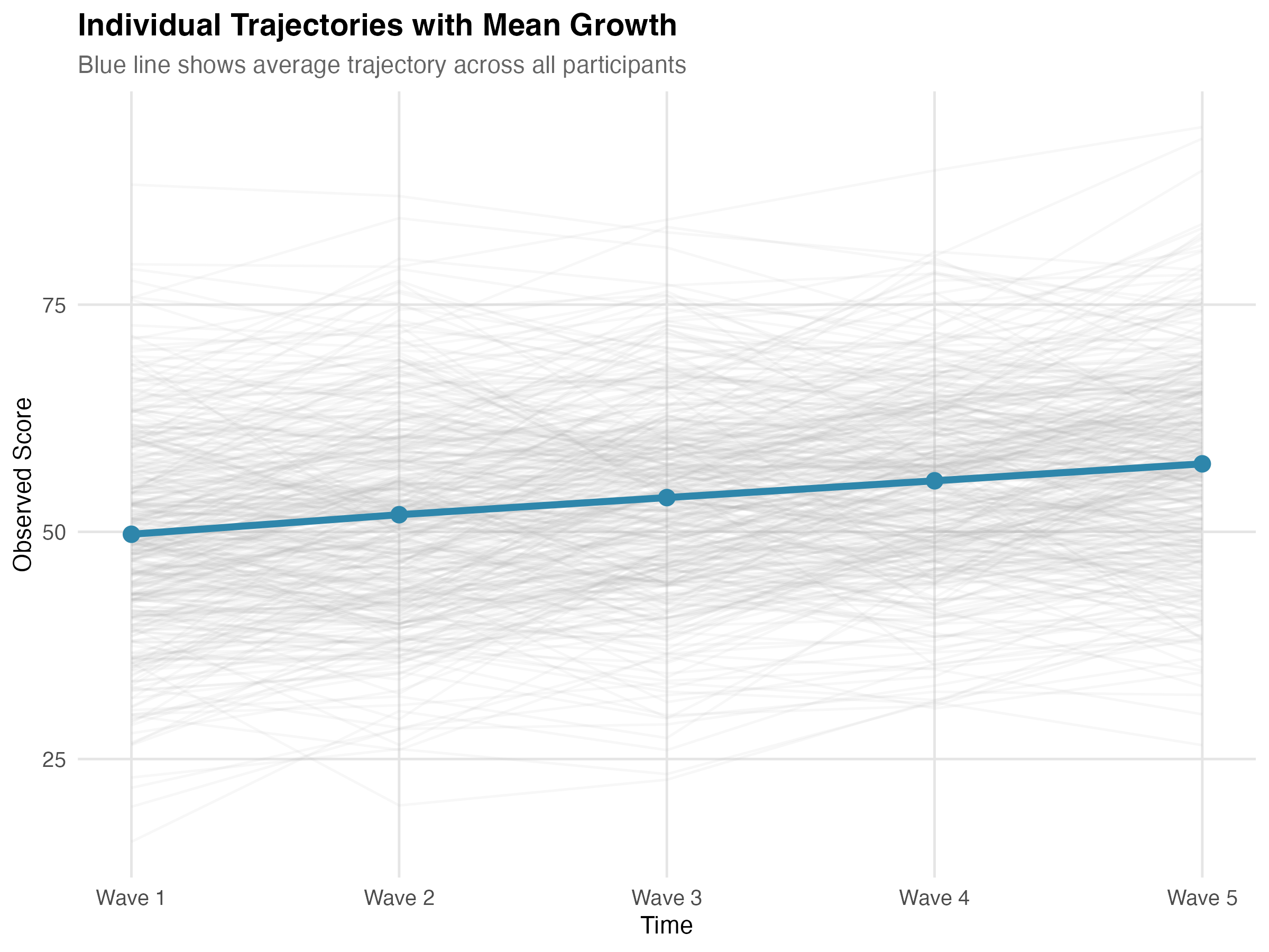
Figure: Individual trajectories (gray) with mean trajectory overlay (blue). The upward trend shows positive average growth; the spread shows individual differences.

✅ Checkpoint: Your plot should show upward-trending lines with visible spread at baseline and a "fan" pattern over time.

Step 4: Fit Models

No-Growth Model (Baseline)

Fit a constrained linear model with no growth—slope mean and variance fixed to zero:

model_nogrowth <- '
  intercept =~ 1*y1 + 1*y2 + 1*y3 + 1*y4 + 1*y5
  slope     =~ 0*y1 + 1*y2 + 2*y3 + 3*y4 + 4*y5

  # Constrain slope to "no growth"
  slope ~ 0*1            # mean(slope) = 0
  slope ~~ 0*slope       # var(slope) = 0
  intercept ~~ 0*slope   # cov(i, s) = 0
'

fit_nogrowth <- growth(model_nogrowth, data = data_wide,
                       missing = "fiml")

Note: This model is nested within the linear growth model, allowing a valid likelihood ratio test.

Linear Growth Model

Add the slope factor:

model_linear <- '
  intercept =~ 1*y1 + 1*y2 + 1*y3 + 1*y4 + 1*y5
  slope     =~ 0*y1 + 1*y2 + 2*y3 + 3*y4 + 4*y5
'

fit_linear <- growth(model_linear, data = data_wide,
                     missing = "fiml")

Note: We specify missing = "fiml" explicitly—good practice even when data are complete. For real data with potential non-normality, add estimator = "MLR" for robust standard errors.

Linear Growth with Equal Residuals

Test whether residual variances can be constrained equal:

model_linear_eq <- '
  intercept =~ 1*y1 + 1*y2 + 1*y3 + 1*y4 + 1*y5
  slope     =~ 0*y1 + 1*y2 + 2*y3 + 3*y4 + 4*y5

  # Constrain residual variances to equality
  y1 ~~ rv*y1
  y2 ~~ rv*y2
  y3 ~~ rv*y3
  y4 ~~ rv*y4
  y5 ~~ rv*y5
'

fit_linear_eq <- growth(model_linear_eq, data = data_wide,
                        missing = "fiml")

Step 5: Compare Models

Is there growth?

anova(fit_nogrowth, fit_linear)

✅ Confirm: Δχ² should be significant (p < .001). This means linear growth improves fit over a flat trajectory (no-growth model).

Are equal residual variances justified?

anova(fit_linear_eq, fit_linear)

Use anova(constrained, unconstrained) so the Δχ² tests the relaxation of constraints.

✅ Confirm: If p > .05, equality is not rejected; prefer the simpler constrained model.

Information criteria

data.frame(
  Model = c("No-growth", "Linear", "Linear (equal resid)"),
  AIC = c(AIC(fit_nogrowth), AIC(fit_linear), AIC(fit_linear_eq)),
  BIC = c(BIC(fit_nogrowth), BIC(fit_linear), BIC(fit_linear_eq))
) %>%
  mutate(across(where(is.numeric), \(x) round(x, 1)))
  # Note: R < 4.1 use function(x) instead of \(x)

✅ Confirm: Lower AIC/BIC = better fit. Linear models should beat no-growth.

Step 6: Check Diagnostics

Before interpreting results, verify model fit and check for problems.

Fit Indices

fitmeasures(fit_linear, c("chisq", "df", "pvalue", "cfi", "rmsea", "srmr"))

✅ Check fit indices:

CFI > .95 ✓
RMSEA < .08 ✓
SRMR < .08 ✓

With small df, RMSEA can be unstable; interpret alongside CFI and SRMR.

See Reference for threshold details.

Modification Indices

modindices(fit_linear, sort = TRUE, minimum.value = 10)

What to look for:

Residual covariances (e.g., y2 ~~ y3): May indicate autocorrelation
Large values (>10) suggest localized misfit
Cross-loadings usually shouldn't be freed in LGCM

Consider multiplicity and substantive plausibility; avoid chasing small local improvements.

✅ Checkpoint: Few or no modification indices >10 indicates good specification.

Residual Correlations

resid(fit_linear, type = "cor")$cor %>% round(3)

Values should be near zero (|r| < 0.10). Large residual correlations mean the model doesn't fully capture those relationships. Thresholds like |r| < .10 are sample-size dependent; in large N, also inspect SEs/tests of residuals.

Check for Problematic Estimates

parameterEstimates(fit_linear) %>%
  filter(op == "~~") %>%
  select(lhs, rhs, est, se) %>%
  mutate(flag = ifelse(est < 0, "NEGATIVE", ""))

Red flags:

Negative variances (Heywood cases): Model misspecified or sample too small
Very large SEs (SE > estimate): Parameter poorly identified
Variances at exactly zero: May need constraints

Heywood case remedies:

Try estimator = "MLR" and/or rescale time to reduce collinearity
Temporarily constrain problematic residual variances to a small positive lower bound while diagnosing

✅ Confirm: All variance estimates should be positive. If any are negative, see Troubleshooting.

Step 7: Interpret Results

summary(fit_linear, fit.measures = TRUE, standardized = TRUE)

Compare Estimates to True Values

Parameter	Estimate	SE	True Value
Intercept mean	49.82	0.51	50
Slope mean	2.04	0.06	2
Intercept variance	98.34	8.12	100
Slope variance	0.97	0.12	1
I-S covariance	-1.89	0.62	-2
Residual variance	24.56	1.23	25

Values shown are illustrative from one simulated run; your numbers will differ with seed, RNG, and package versions (even with the same seed).

✅ Success: Estimates closely recover the true population parameters. This confirms the model is working correctly.

Interpret Each Parameter

Intercept mean ≈ 50: Average score at Wave 1
Slope mean ≈ 2: Average increase per wave
Intercept variance ≈ 100 (SD ≈ 10): People differed in starting levels
Slope variance ≈ 1 (SD ≈ 1): People differed in growth rates
I-S covariance ≈ -2: Higher starters grew slightly slower (see correlation below)

Intercept-Slope Correlation

Convert the covariance to a correlation for interpretability:

cov_is <- -1.89
var_i <- 98.34
var_s <- 0.97

r_is <- cov_is / sqrt(var_i * var_s)
r_is  # ≈ -0.19

The correlation of -0.19 is small—higher starters grew slower, but most still improved.

Proportion with Positive Slopes

A positive slope mean doesn't mean everyone improved. Check:

slope_mean <- 2.04
slope_sd <- sqrt(0.97)  # ≈ 0.98

# P(slope > 0) — theoretical
pnorm(0, mean = slope_mean, sd = slope_sd, lower.tail = FALSE)
# ≈ 0.98

# Empirical check using factor scores (posterior means)
fs <- lavPredict(fit_linear, type = "lv")
mean(fs[, "slope"] > 0)
# Should be close to the theoretical value

✅ Checkpoint: ~98% of participants had positive slopes. With slope mean = 2 and SD ≈ 1, almost everyone improved. The empirical proportion from factor scores should match the theoretical pnorm() result.

Variance Explained

inspect(fit_linear, "r2")

Expected R² values: 0.80–0.89 across waves.

Interpretation: The trajectory (intercept + slope) explains 80–89% of variance at each wave. The remaining 10–20% is residual variance (measurement error, occasion-specific factors).

✅ Check: R² values of 0.70–0.90 are typical for well-fitting LGCMs.

Written Summary

We estimated a linear latent growth model for 400 participants across 5 waves. The model fit well (χ²(10) = 12.35, p = .26; CFI = 0.998; RMSEA = 0.024; SRMR = 0.025).

On average, participants started at 49.82 (SE = 0.51) and increased by 2.04 units per wave (SE = 0.06), both p < .001. Significant individual differences emerged in starting levels (variance = 98.34, SD ≈ 10) and growth rates (variance = 0.97, SD ≈ 1). The negative intercept-slope covariance (-1.89, p = .002, r ≈ -0.19) indicates that participants who started higher grew slightly slower.

Complete Script

# ============================================
# LGCM Complete Worked Example
# ============================================

library(tidyverse)
library(lavaan)
library(MASS)
set.seed(2024)

# Simulate data
n <- 400
psi <- matrix(c(100, -2, -2, 1), nrow = 2)
factors <- mvrnorm(n, mu = c(50, 2), Sigma = psi)

data_wide <- tibble(id = 1:n) %>%
  mutate(
    int = factors[,1], slp = factors[,2],
    y1 = int + slp*0 + rnorm(n, 0, 5),
    y2 = int + slp*1 + rnorm(n, 0, 5),
    y3 = int + slp*2 + rnorm(n, 0, 5),
    y4 = int + slp*3 + rnorm(n, 0, 5),
    y5 = int + slp*4 + rnorm(n, 0, 5)
  ) %>% select(id, y1:y5)

# Visualize
data_long <- data_wide %>%
  pivot_longer(y1:y5, names_to = "wave", values_to = "y") %>%
  mutate(time = as.numeric(gsub("y", "", wave)) - 1)

ggplot(data_long, aes(x = time, y = y, group = id)) +
  geom_line(alpha = 0.15) +
  theme_minimal() +
  labs(title = "Individual Trajectories")

# Fit models
model_nogrowth <- '
  intercept =~ 1*y1 + 1*y2 + 1*y3 + 1*y4 + 1*y5
  slope     =~ 0*y1 + 1*y2 + 2*y3 + 3*y4 + 4*y5
  slope ~ 0*1; slope ~~ 0*slope; intercept ~~ 0*slope
'
model_lin <- '
  intercept =~ 1*y1 + 1*y2 + 1*y3 + 1*y4 + 1*y5
  slope     =~ 0*y1 + 1*y2 + 2*y3 + 3*y4 + 4*y5
'

fit_nogrowth <- growth(model_nogrowth, data = data_wide, missing = "fiml")
fit_lin <- growth(model_lin, data = data_wide, missing = "fiml")

# Compare and summarize
anova(fit_nogrowth, fit_lin)
summary(fit_lin, fit.measures = TRUE, standardized = TRUE)
fitmeasures(fit_lin, c("chisq", "df", "pvalue", "cfi", "rmsea", "srmr"))
inspect(fit_lin, "r2")

Adapt to Your Data

To use this workflow with your own dataset:

1. Read and Prepare Data

library(readr)
library(dplyr)

# Read your data (wide format: one row per person)
data_wide <- read_csv("my_longitudinal_data.csv") %>%
  select(id, outcome_t1, outcome_t2, outcome_t3, outcome_t4, outcome_t5)

2. Update Variable Names

Replace y1–y5 with your variable names:

model <- '
  intercept =~ 1*outcome_t1 + 1*outcome_t2 + 1*outcome_t3 + 1*outcome_t4 + 1*outcome_t5
  slope     =~ 0*outcome_t1 + 1*outcome_t2 + 2*outcome_t3 + 3*outcome_t4 + 4*outcome_t5
'

fit <- growth(model, data = data_wide, missing = "fiml")
summary(fit, fit.measures = TRUE, standardized = TRUE)

3. Adjust Time Coding (if needed)

If waves are unequally spaced, adjust slope loadings to reflect actual time. For example, measurements at baseline, 1, 3, 6, and 12 months:

model <- '
  intercept =~ 1*y_0mo + 1*y_1mo + 1*y_3mo + 1*y_6mo + 1*y_12mo
  slope     =~ 0*y_0mo + 1*y_1mo + 3*y_3mo + 6*y_6mo + 12*y_12mo
'
# Now slope = change per month

Rescaling time (e.g., months → years) rescales the slope mean and variance (per-unit); choose units that are meaningful for interpretation.

✅ Checkpoint: Once your basic model runs, layer on diagnostics, model comparisons, and predictors exactly as shown above.

Next Steps

Need syntax or thresholds? → Reference
Hit an error? → Reference: Troubleshooting
Back to overview → LGCM Guide